Buckling of a heated von-Kármán plate
This demo is implemented in the single Python file demo_von-karman-mansfield.py.
This demo program solves the von-Kármán equations on a circular plate with a lenticular cross section free on the boundary. The plate is heated, causing it to bifurcate. Bifurcation occurs with a striking shape transition: before the critical threshold the plate assumes a cup-shaped configurations (left); above it tends to a cylindrical shape (right). An analytical solution has been found by Mansfield, see [1].
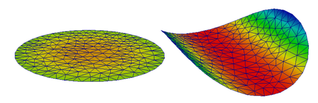
Pre-critical and post-critical plate configuration.
The standard von-Kármán theory gives rise to a fourth-order PDE which requires the transverse displacement field \(w\) to be sought in the space \(H^2(\Omega)\). We relax this requirement in the same manner as the Kirchoff-Love plate theory can be relaxed to the Reissner-Mindlin theory, resulting in seeking a transverse displacement field \(w\) in \(H^1(\Omega)\) and a rotation field \(\theta\) in \([H^2(\Omega)]^2\). To alleviate the resulting shear- and membrane-locking issues we use Partial Selective Reduced Integration (PSRI), see [2].
To follow this demo you should know how to:
- Define a
MixedElementand aFunctionSpacefrom it. - Write variational forms using the Unified Form Language.
- Automatically derive Jabobian and residuals using
derivative(). - Apply Dirichlet boundary conditions using
DirichletBCandapply(). - Assemble forms using
assemble().
This demo then illustrates how to:
- Define the Reissner-Mindlin-von-Kármán plate equations using UFL.
- Use the PSRI approach to simultaneously cure shear- and membrane-locking issues.
We start with importing the required modules, setting matplolib as
plotting backend, and generically set the integration order to 4 to
avoid the automatic setting of FEniCS which would lead to unreasonably
high integration orders for complex forms.
from dolfin import *
from fenics_shells import *
import mshr
import numpy as np
import matplotlib.pyplot as plt

parameters["form_compiler"]["quadrature_degree"] = 4
The mid-plane of the plate is a circular domain with radius \(a = 1\). We
generate a mesh of the domain using the package mshr:
a = 1.
ndiv = 8
domain_area = np.pi*a**2

centre = Point(0.,0.)

geom = mshr.Circle(centre, a)
mesh = mshr.generate_mesh(geom, ndiv)
The lenticular thinning of the plate can be modelled directly through the thickness parameter in the plate model:
t = 1E-2
ts = interpolate(Expression('t*(1.0 - (x[0]*x[0] + x[1]*x[1])/(a*a))', t=t, a=a, degree=2), FunctionSpace(mesh, 'CG', 2))
We assume the plate is isotropic with constant material parameters, Young’s modulus \(E\), Poisson’s ratio \(\nu\); shear correction factor \(\kappa\):
E = Constant(1.0)
nu = Constant(0.3)
kappa = Constant(5.0/6.0)
Then, we compute the (scaled) membrane, \(A/t^3\), bending, \(D/t^3\), and shear, \(S/t^3\), plate elastic stiffnesses:
A = (E*ts/t**3/(1. - nu**2))*as_tensor([[1., nu, 0.],[nu, 1., 0.],[0., 0., (1. - nu)/2]])
D = (E*ts**3/t**3/(12.*(1. - nu**2)))*as_tensor([[1., nu, 0.],[nu, 1., 0.],[0., 0., (1. - nu)/2]])
S = E*kappa*ts/t**3/(2*(1. + nu))
We use a \(CG_2\) element for the in-plane and transverse displacements \(u\) and \(w\), and the enriched element \([CG_1 + B_3]\) for the rotations \(\theta\). We collect the variables in the state vector \(q =(u,w,\theta)\):
P1 = FiniteElement("Lagrange", triangle, degree = 1)
P2 = FiniteElement("Lagrange", triangle, degree = 2)
bubble = FiniteElement("B", triangle, degree = 3)
enriched = P1 + bubble

element = MixedElement([VectorElement(P2, dim=2), P2, VectorElement(enriched, dim=2)])

Q = FunctionSpace(mesh, element)
Then, we define Function, TrialFunction and TestFunction objects to express the variational forms and we split them into each individual component function:
q_, q, q_t = Function(Q), TrialFunction(Q), TestFunction(Q)
v_, w_, theta_ = split(q_)
The membrane strain tensor \(e\) for the von-Kármán plate takes into account the nonlinear contribution of the transverse displacement in the approximate form:
which can be expressed in UFL as:
e = sym(grad(v_)) + 0.5*outer(grad(w_), grad(w_))
The membrane energy density \(\psi_m\) is a quadratic function of the membrane strain
tensor \(e\). For convenience, we use our function strain_to_voigt() to express \(e\) in Voigt notation \(e_V = \{e_1, e_2, 2 e_{12}\}\):
ev = strain_to_voigt(e)
psi_m = 0.5*dot(A*ev, ev)
The bending strain tensor \(k\) and shear strain vector \(\gamma\) are identical to the standard Reissner-Mindlin model. The shear energy density \(\psi_s\) is a quadratic function of the shear strain vector:
gamma = grad(w_) - theta_
psi_s = 0.5*dot(S*gamma, gamma)
The bending energy density \(\psi_b\) is a quadratic function of the bending strain tensor. Here, the temperature profile on the plate is not modelled directly. Instead, it gives rise to an inelastic (initial) bending strain tensor \(k_T\) which can be incoporated directly in the Lagrangian:
k_T = as_tensor(Expression((("c/imp","0.0"),("0.0","c*imp")), c=1., imp=.999,  degree=0))
k = sym(grad(theta_)) - k_T
kv = strain_to_voigt(k)
psi_b = 0.5*dot(D*kv, kv)
Note
The standard von-Kármán model can be recovered by substituting in the Kirchoff constraint \(\theta = \nabla w\).
Shear- and membrane-locking are treated using the partial reduced selective integration proposed by Arnold and Brezzi, see [2]. In this approach shear and membrane energy are splitted as a sum of two contributions weighted by a factor \(\alpha\). One of the two contributions is integrated with a reduced integration. We use \(2\times 2\)-points Gauss integration for a portion \(1-\alpha\) of the energy, whilst the rest is integrated with a \(4\times 4\) scheme. We adopt an optimized weighting factor \(\alpha=(t/h)^2\), where \(h\) is the mesh size.:
dx_h = dx(metadata={'quadrature_degree': 2})
h = CellDiameter(mesh)
alpha = project(t**2/h**2, FunctionSpace(mesh,'DG',0))

Pi_PSRI = psi_b*dx + alpha*psi_m*dx + alpha*psi_s*dx + (1.0 - alpha)*psi_s*dx_h + (1.0 - alpha)*psi_m*dx_h
Then, we compute the total elastic energy and its first and second derivatives:
Pi = Pi_PSRI
dPi = derivative(Pi, q_, q_t)
J = derivative(dPi, q_, q)
This problem is a pure Neumann problem. This leads to a nullspace in the solution. To remove this nullspace, we fix all the variables in the central point of the plate and the displacements in the \(x_0\) and \(x_1\) direction at \((0, a)\) and \((a, 0)\), respectively:
zero_v1 = project(Constant((0.)), Q.sub(0).sub(0).collapse())
zero_v2 = project(Constant((0.)), Q.sub(0).sub(1).collapse())
zero = project(Constant((0.,0.,0.,0.,0.)), Q)

bc = DirichletBC(Q, zero, "near(x[0], 0.) and near(x[1], 0.)", method="pointwise")
bc_v1 = DirichletBC(Q.sub(0).sub(0), zero_v1, "near(x[0], 0.) and near(x[1], 1.)", method="pointwise")
bc_v2 = DirichletBC(Q.sub(0).sub(1), zero_v2, "near(x[0], 1.) and near(x[1], 0.)", method="pointwise")
bcs = [bc, bc_v1, bc_v2]
Then, we define the nonlinear variational problem and the solver settings:
init = Function(Q)
q_.assign(init)
problem = NonlinearVariationalProblem(dPi, q_, bcs, J = J)
solver = NonlinearVariationalSolver(problem)
solver.parameters["newton_solver"]["absolute_tolerance"] = 1E-8
Finally, we choose the continuation steps (the critical loading c_cr is taken from the Mansfield analytical solution [1]):
c_cr = 0.0516
cs = np.linspace(0.0, 1.5*c_cr, 30)
and we solve as usual:
defplots_dir = "output/3dplots-psri/"
file = File(defplots_dir + "sol.pvd")

ls_kx = []
ls_ky = []
ls_kxy = []
ls_kT = []

for count, i in enumerate(cs):
    k_T.c = i
    solver.solve()
    v_h, w_h, theta_h = q_.split(deepcopy=True)
To visualise the solution we assemble the bending strain tensor:
K_h = project(sym(grad(theta_h)), TensorFunctionSpace(mesh, 'DG', 0))
we compute the average bending strain:
Kxx = assemble(K_h[0,0]*dx)/domain_area
Kyy = assemble(K_h[1,1]*dx)/domain_area
Kxy = assemble(K_h[0,1]*dx)/domain_area

ls_kT.append(i)
ls_kx.append(Kxx)
ls_ky.append(Kyy)
ls_kxy.append(Kxy)
and output the results at each continuation step:
v1_h, v2_h = v_h.split()
u_h = as_vector([v1_h, v2_h, w_h])
u_h_pro = project(u_h, VectorFunctionSpace(mesh, 'CG', 1, dim=3))
u_h_pro.rename("q_","q_")
file << u_h_pro
Finally, we plot the average curvatures as a function of the inelastic curvature:
fig = plt.figure(figsize=(5.0, 5.0/1.648))
plt.plot(ls_kT, ls_kx, "o", color='orange', label=r"$k_{1h}$")
plt.plot(ls_kT, ls_ky, "x", color='red', label=r"$k_{2h}$")
plt.xlabel(r"inelastic curvature $\eta$")
plt.ylabel(r"curvature $k_{1,2}$")
plt.legend()
plt.tight_layout()
plt.savefig("psri-%s.png"%ndiv)
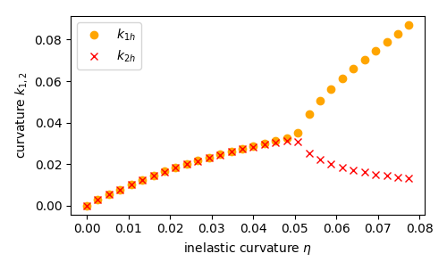
Comparison with the analytical solution.
Unit testing
import pytest
@pytest.mark.skip
def test_close():
    pass
References
[1] E. H. Mansfield, “Bending, Buckling and Curling of a Heated Thin Plate. Proceedings of the Royal Society of London A: Mathematical, Physical and Engineering Sciences. Vol. 268. No. 1334. The Royal Society, 1962.
[2] D. Arnold and F.Brezzi, Mathematics of Computation, 66(217): 1-14, 1997. https://www.ima.umn.edu/~arnold//papers/shellelt.pdf