Clamped semi-cylindrical Naghdi shell under point load
This demo is implemented in the single Python file
demo_nonlinear-naghdi-cylindrical.py.
This demo program solves the nonlinear Naghdi shell equations for a semi-cylindrical shell loaded by a point force. This problem is a standard reference for testing shell finite element formulations, see [1]. The numerical locking issue is cured using enriched finite element including cubic bubble shape functions and Partial Selective Reduced Integration [2].
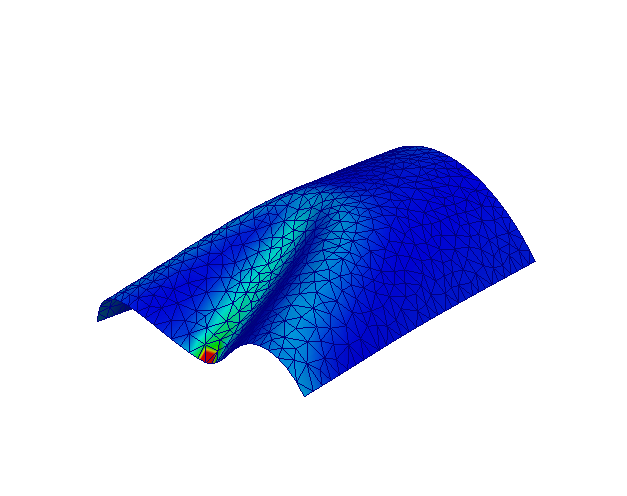
Shell deformed configuration.
To follow this demo you should know how to:
- Define a
MixedElementand aFunctionSpacefrom it. - Write variational forms using the Unified Form Language.
- Automatically derive Jacobian and residuals using derivative().
- Apply Dirichlet boundary conditions using DirichletBC and apply().
- Solve non-linear problems using NonlinearProblem.
- Output data to XDMF files with XDMFFile.
This demo then illustrates how to:
- Define and solve a nonlinear Naghdi shell problem with a curved stress-free configuration given as analytical expression in terms of two curvilinear coordinates.
- Use the PSRI approach to simultaneously cure shear- and membrane-locking issues.
We start with importing the required modules, setting matplolib as
plotting backend, and generically set the integration order to 4 to
avoid the automatic setting of FEniCS which would lead to unreasonably
high integration orders for complex forms.
import os, sys

import numpy as np
import matplotlib.pyplot as plt

from dolfin import *
from ufl import Index
from mshr import *
from mpl_toolkits.mplot3d import Axes3D

parameters["form_compiler"]["quadrature_degree"] = 4

output_dir = "output/"
if not os.path.exists(output_dir):
    os.makedirs(output_dir)
We consider a semi-cylindrical shell of radius \(\rho\) and axis length \(L\). The shell is made of a linear elastic isotropic homogeneous material with Young modulus \(E\) and Poisson ratio \(\nu\). The (uniform) shell thickness is denoted by \(t\). The Lamé moduli \(\lambda\), \(\mu\) are introduced to write later the 2D constitutive equation in plane-stress:
rho = 1.016
L = 3.048
E, nu = 2.0685E7, 0.3
mu = E/(2.0*(1.0 + nu))
lmbda = 2.0*mu*nu/(1.0 - 2.0*nu)
t = Constant(0.03)
The midplane of the initial (stress-free) configuration \({\mit \Phi_0}\) of the shell is given in the form of an analytical expression
in terms of the curvilinear coordinates \(x\). In the specific case we adopt the cylindrical coordinates \(x_0\) and \(x_1\) representing the angular and axial coordinates, respectively. Hence we mesh the two-dimensional domain \(\omega \equiv [0,L_y] \times [-\pi/2,\pi/2]\).
P1, P2 = Point(-np.pi/2., 0.), Point(np.pi/2., L)
ndiv = 21
mesh = generate_mesh(Rectangle(P1, P2), ndiv)
plot(mesh); plt.xlabel(r"$x_0$"); plt.ylabel(r"$x_1$")
plt.savefig("output/mesh.png")
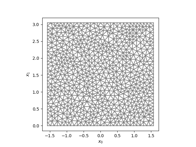
Discretisation of the parametric domain.
We provide the analytical expression of the initial shape as an
Expression that we represent on a suitable FunctionSpace (here
\(P_2\), but other are choices are possible):
initial_shape = Expression(('r*sin(x[0])','x[1]','r*cos(x[0])'), r=rho, degree = 4)
V_phi =  FunctionSpace(mesh, VectorElement("P", triangle, degree = 2, dim = 3))
phi0 = project(initial_shape, V_phi)
Given the midplane, we define the corresponding unit normal as below and project on a suitable function space (here \(P_1\) but other choices are possible):
def normal(y):
    n = cross(y.dx(0), y.dx(1))
    return n/sqrt(inner(n,n))

V_normal = FunctionSpace(mesh, VectorElement("P", triangle, degree = 1, dim = 3))
n0 = project(normal(phi0), V_normal)
The kinematics of the Nadghi shell model is defined by the following vector fields :
- \(\phi\): the position of the midplane, or the displacement from the reference configuration \(u = \phi - \phi_0\):
- \(d\): the director, a unit vector giving the orientation of the microstructure
We parametrize the director field by two angles, which correspond to spherical coordinates, so as to explicitly resolve the unit norm constraint (see [3]):
def director(beta):
    return as_vector([sin(beta[1])*cos(beta[0]), -sin(beta[0]), cos(beta[1])*cos(beta[0])])
We assume that in the initial configuration the director coincides with the normal. Hence, we can define the angles \(\beta\): for the initial configuration as follows:
beta0_expression = Expression(["atan2(-n[1], sqrt(pow(n[0],2) + pow(n[2],2)))",
                               "atan2(n[0],n[2])"], n = n0, degree=4)

V_beta = FunctionSpace(mesh, VectorElement("P", triangle, degree = 2, dim = 2))
beta0 = project(beta0_expression, V_beta)
The director in the initial configuration is then written as
d0 = director(beta0)
We can visualize the shell shape and its normal with this utility function:
def plot_shell(y,n=None):
    y_0, y_1, y_2 = y.split(deepcopy=True)
    fig = plt.figure()
    ax = fig.gca(projection='3d')
    ax.plot_trisurf(y_0.compute_vertex_values(),
                    y_1.compute_vertex_values(),
                    y_2.compute_vertex_values(),
                    triangles=y.function_space().mesh().cells(),
                    linewidth=1, antialiased=True, shade = False)
    if n:
        n_0, n_1, n_2 = n.split(deepcopy=True)
        ax.quiver(y_0.compute_vertex_values(),
              y_1.compute_vertex_values(),
              y_2.compute_vertex_values(),
              n_0.compute_vertex_values(),
              n_1.compute_vertex_values(),
              n_2.compute_vertex_values(),
              length = .2, color = "r")
    ax.view_init(elev=20, azim=80)
    plt.xlabel(r"$x_0$")
    plt.ylabel(r"$x_1$")
    plt.xticks([-1,0,1])
    plt.yticks([0,pi/2])
    return ax

plot_shell(phi0, project(d0, V_normal))
plt.savefig("output/initial_configuration.png")
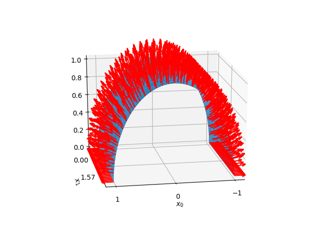
Shell initial shape and normal.
In our 5-parameter Naghdi shell model the configuration of the shell is assigned by
- the 3-component vector field \(u\): representing the displacement with respect to the initial configuration \(\phi_0\):
- the 2-component vector field \(\beta\): representing the angle variation of the director \(d\): with respect to the initial configuration
Following [1], we use a \([P_2 + B_3]\) element for \(u\) and a \([CG_2]^2\) element for \(beta\), and collect them in the state vector \(q = (u, \beta)\):
P2 = FiniteElement("Lagrange", triangle, degree = 2)
bubble = FiniteElement("B", triangle, degree = 3)
enriched = P2 + bubble

element = MixedElement([VectorElement(enriched, dim=3), VectorElement(P2, dim=2)])

Q = FunctionSpace(mesh, element)
Then, we define Function, TrialFunction and TestFunction objects to express the variational forms and we split them into each individual component function:
q_, q, q_t = Function(Q), TrialFunction(Q), TestFunction(Q)
u_, beta_ = split(q_)
The gradient of the transformation and the director in the current configuration are given by:
F = grad(u_) + grad(phi0)
d = director(beta_ + beta0)
With the following definition of the natural metric and curvature
a0 = grad(phi0).T*grad(phi0)
b0 = -0.5*(grad(phi0).T*grad(d0) + grad(d0).T*grad(phi0))
The membrane, bending, and shear strain measures of the Naghdi model are defined by:
e = lambda F: 0.5*(F.T*F - a0)
k = lambda F, d: -0.5*(F.T*grad(d) + grad(d).T*F) - b0
gamma = lambda F, d: F.T*d - grad(phi0).T*d0
Using curvilinear coordinates, and denoting by a0_contra the
contravariant components of the metric tensor \(a_0^{\alpha\beta}\) (in the initial curved configuration)
the constitutive equation is written in terms of the matrix \(A\) below,
representing the contravariant components of the constitutive tensor
for isotropic elasticity in plane stress (see e.g. [4]).
We use the index notation offered by UFL to express
operations between tensors:
a0_contra = inv(a0)
j0 = det(a0)

i, j, l, m = Index(), Index(), Index(), Index()
A_ = as_tensor((((2.0*lmbda*mu)/(lmbda + 2.0*mu))*a0_contra[i,j]*a0_contra[l,m]
                + 1.0*mu*(a0_contra[i,l]*a0_contra[j,m] + a0_contra[i,m]*a0_contra[j,l]))
                ,[i,j,l,m])
The normal stress \(N\), bending moment \(M\), and shear stress \(T\) tensors are (they are purely Lagrangian stress measures, similar to the so called 2nd Piola stress tensor in 3D elasticity):
N = as_tensor(t*A_[i,j,l,m]*e(F)[l,m], [i,j])
M = as_tensor((t**3/12.0)*A_[i,j,l,m]*k(F,d)[l,m],[i,j])
T = as_tensor(t*mu*a0_contra[i,j]*gamma(F,d)[j], [i])
Hence, the contributions to the elastic energy density due to membrane, \(\psi_m\), bending, \(\psi_b\), and shear, \(\psi_s\) are (they are per unit surface in the initial configuration):
psi_m = 0.5*inner(N, e(F))
psi_b = 0.5*inner(M, k(F,d))
psi_s = 0.5*inner(T, gamma(F,d))
Shear and membrane locking is treated using the partial reduced selective integration proposed in Arnold and Brezzi [2]. In this approach shear and membrane energy are splitted as a sum of two contributions weighted by a factor \(\alpha\). One of the two contributions is integrated with a reduced integration. While [1] suggests a 1-point reduced integration, we observed that this leads to spurious modes in the present case. We use then \(2\times 2\)-points Gauss integration for a portion \(1-\alpha\) of the energy, whilst the rest is integrated with a \(4\times 4\) scheme. We further refine the approach of [1] by adopting an optimized weighting factor \(\alpha=(t/h)^2\), where \(h\) is the mesh size.
dx_h = dx(metadata={'quadrature_degree': 2})
h = CellDiameter(mesh)
alpha = project(t**2/h**2, FunctionSpace(mesh,'DG',0))

Pi_PSRI = psi_b*sqrt(j0)*dx + alpha*psi_m*sqrt(j0)*dx + alpha*psi_s*sqrt(j0)*dx + (1.0 - alpha)*psi_s*sqrt(j0)*dx_h + (1.0 - alpha)*psi_m*sqrt(j0)*dx_h
Hence the total elastic energy and its first and second derivatives are
Pi = Pi_PSRI
dPi = derivative(Pi, q_, q_t)
J = derivative(dPi, q_, q)
The boundary conditions prescribe a full clamping on the top boundary, while on the left and the right side the normal component of the rotation and the transverse displacement are blocked:
up_boundary = lambda x, on_boundary: x[1] <= 1.e-4 and on_boundary
leftright_boundary = lambda x, on_boundary: near(abs(x[0]), pi/2., 1.e-6)  and on_boundary

bc_clamped = DirichletBC(Q, project(q_, Q), up_boundary)
bc_u = DirichletBC(Q.sub(0).sub(2), project(Constant(0.), Q.sub(0).sub(2).collapse()), leftright_boundary)
bc_beta = DirichletBC(Q.sub(1).sub(1), project(q_[4], Q.sub(1).sub(0).collapse()), leftright_boundary)
bcs = [bc_clamped, bc_u, bc_beta]
The loading is exerted by a point force applied at the midpoint of the bottom boundary.
This is implemented using the PointSource in FEniCS and
defining a custom NonlinearProblem:
class NonlinearProblemPointSource(NonlinearProblem):

    def __init__(self, L, a, bcs):
        NonlinearProblem.__init__(self)
        self.L = L
        self.a = a
        self.bcs = bcs
        self.P = 0.0

    def F(self, b, x):
        assemble(self.L, tensor=b)
        point_source = PointSource(self.bcs[0].function_space().sub(0).sub(2), Point(0.0, L), self.P)
        point_source.apply(b)
        for bc in self.bcs:
            bc.apply(b, x)

    def J(self, A, x):
        assemble(self.a, tensor=A)
        for bc in self.bcs:
            bc.apply(A, x)

problem = NonlinearProblemPointSource(dPi, J, bcs)
We use a standard Newton solver and setup the files for the writing the results to disk:
solver = NewtonSolver()
output_dir = "output/"
file_phi = File(output_dir + "configuration.pvd")
file_energy = File(output_dir + "energy.pvd")
Finally, we can solve the quasi-static problem, incrementally increasing the loading from \(0\) to \(2000\) N:
P_values = np.linspace(0.0, 2000.0, 40)
displacement = 0.*P_values
q_.assign(project(Constant((0,0,0,0,0)), Q))

for (i, P) in enumerate(P_values):
    problem.P = P
    (niter,cond) = solver.solve(problem, q_.vector())

    phi = project(u_ + phi0, V_phi)
    displacement[i] = phi(0.0, L)[2] - phi0(0.0, L)[2]

    phi.rename("phi", "phi")
    file_phi << (phi, P)
    print("Increment %d of %s. Converged in %2d iterations. P:  %.2f, Displ: %.2f" %(i, P_values.size,niter,P, displacement[i]))

    en_function = project(psi_m + psi_b + psi_s, FunctionSpace(mesh, 'Lagrange', 1))
    en_function.rename("Elastic Energy", "Elastic Energy")
    file_energy << (en_function,P)
We can plot the final configuration of the shell:
plot_shell(phi)
plt.savefig("output/finalconfiguration.png")
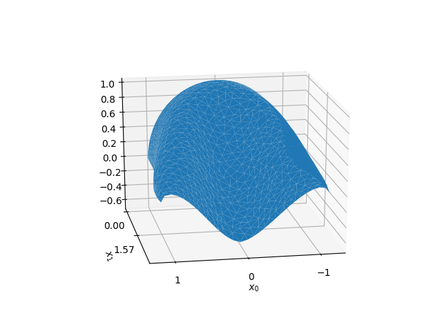
Shell deformed shape.
The results for the transverse displacement at the point of application of the force are validated against a standard reference from the literature, obtained using Abaqus S4R element and a structured mesh of \(40\times 40\) elements, see [1]:
plt.figure()
reference_Sze = np.array([
    1.e-2*np.array([0., 5.421, 16.1, 22.195, 27.657, 32.7, 37.582, 42.633,
    48.537, 56.355, 66.410, 79.810, 94.669, 113.704, 124.751, 132.653,
    138.920, 144.185, 148.770, 152.863, 156.584, 160.015, 163.211,
    166.200, 168.973, 171.505]),
    2000.*np.array([0., .05, .1, .125, .15, .175, .2, .225, .25, .275, .3,
    .325, .35, .4, .45, .5, .55, .6, .65, .7, .75, .8, .85, .9, .95, 1.])
    ])
plt.plot(-np.array(displacement), P_values, label='fenics-shell %s divisions (AB)'%ndiv)
plt.plot(*reference_Sze, "or", label='Sze (Abaqus S4R)')
plt.xlabel("Displacement (mm)")
plt.ylabel("Load (N)")
plt.legend()
plt.grid()
plt.savefig("output/comparisons.png")
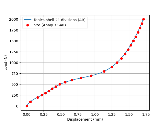
Comparison with reference solution.
References
[1] K. Sze, X. Liu, and S. Lo. Popular benchmark problems for geometric nonlinear analysis of shells. Finite Elements in Analysis and Design, 40(11):1551 – 1569, 2004.
[2] D. Arnold and F.Brezzi, Mathematics of Computation, 66(217): 1-14, 1997. https://www.ima.umn.edu/~arnold//papers/shellelt.pdf
[3] P. Betsch, A. Menzel, and E. Stein. On the parametrization of finite rotations in computational mechanics: A classification of concepts with application to smooth shells. Computer Methods in Applied Mechanics and Engineering, 155(3):273 – 305, 1998.
[4] P. G. Ciarlet. An introduction to differential geometry with applications to elasticity. Journal of Elasticity, 78-79(1-3):1–215, 2005.