Clamped Reissner-Mindlin plate under uniform load
This demo is implemented in the single Python file demo_reissner-mindlin-clamped.py.
This demo program solves the out-of-plane Reissner-Mindlin equations on the unit square with uniform transverse loading with fully clamped boundary conditions. It is assumed the reader understands most of the functionality in the FEniCS Project documented demos.
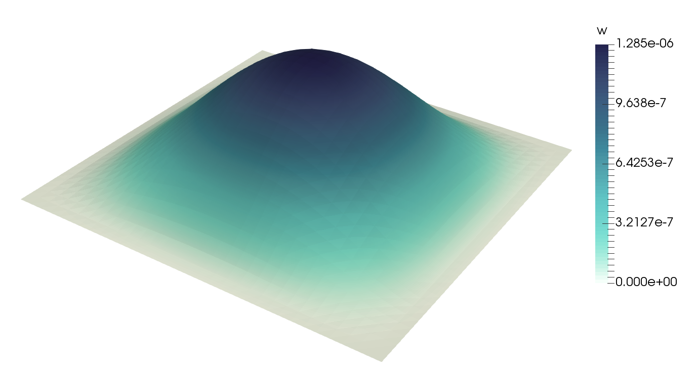
Transverse displacement field \(w\) of the clamped Reissner-Mindlin plate problem scaled by a factor of 250000.
Specifically, you should know how to:
- Define a
MixedElementand aFunctionSpacefrom it. - Write variational forms using the Unified Form Language.
- Automatically derive Jacobian and residuals using
derivative(). - Apply Dirichlet boundary conditions using
DirichletBCandapply(). - Assemble forms using
assemble(). - Solve linear systems using
LUSolver. - Output data to XDMF files with
XDMFFile.
This demo then illustrates how to:
- Define the Reissner-Mindlin plate equations using UFL.
- Define the Durán-Liberman (MITC) reduction operator using UFL. This procedure eliminates the shear-locking problem.
- Use
ProjectedFunctionSpaceandassemble()in FEniCS-Shells to statically condensate two problem variables and assemble a linear system of reduced size. - Reconstruct the variables that were statically condensated using
reconstruct_full_space().
First the dolfin and fenics_shells modules are imported.
The fenics_shells module overrides some standard methods in DOLFIN,
so it should always be import-ed after dolfin:
from dolfin import *
from fenics_shells import *
We then create a two-dimensional mesh of the mid-plane of the plate \(\Omega = [0, 1] \times [0, 1]\):
mesh = UnitSquareMesh(32, 32)
The Durán-Liberman element for the Reissner-Mindlin plate problem consists of second-order vector-valued element for the rotation field \(\theta \in [\mathrm{CG}_2]^2\) and a first-order scalar valued element for the transverse displacement field \(w \in \mathrm{CG}_1\), see [1]. Two further auxilliary fields are also considered, the reduced shear strain \(\gamma_R\), and a Lagrange multiplier field \(p\) which ties together the shear strain calculated from the primal variables \(\gamma = \nabla w - \theta\) and the reduced shear strain \(\gamma_R\). Both \(p\) and \(\gamma_R\) are are discretised in the space \(\mathrm{NED}_1\), the vector-valued Nédélec elements of the first kind. The final element definition is then:
element = MixedElement([VectorElement("Lagrange", triangle, 2),
                        FiniteElement("Lagrange", triangle, 1),
                        FiniteElement("N1curl", triangle, 1),
                        FiniteElement("N1curl", triangle, 1)])
We then pass our element through to the ProjectedFunctionSpace
constructor. As we will see later in this example, we can project out both the
\(p\) and \(\mathrm{NED}_1\) fields at assembly time. We specify this
by passing the argument num_projected_subspaces=2:
Q = ProjectedFunctionSpace(mesh, element, num_projected_subspaces=2)
From Q we can then extract the full space Q_F, which consists of all
four function fields, collected in the state vector \(q=(\theta, w, \gamma_R, p)\).
Q_F = Q.full_space
In contrast the projected space Q only holds the two primal problem fields
\((\theta, w)\).
Using only the full function space object Q_F we setup our variational
problem by defining the Lagrangian of the Reissner-Mindlin plate problem. We
begin by creating a Function and splitting it into each individual
component function:
q_ = Function(Q_F)
theta_, w_, R_gamma_, p_ = split(q_)
q = TrialFunction(Q_F)
q_t = TestFunction(Q_F)
We assume constant material parameters; Young’s modulus \(E\), Poisson’s ratio \(\nu\), shear-correction factor \(\kappa\), and thickness \(t\):
E = Constant(10920.0)
nu = Constant(0.3)
kappa = Constant(5.0/6.0)
t = Constant(0.001)
The bending strain tensor \(k\) for the Reissner-Mindlin model can be expressed in terms of the rotation field \(\theta\):
which can be expressed in UFL as:
k = sym(grad(theta_))
The bending energy density \(\psi_b\) for the Reissner-Mindlin model is a function of the bending strain tensor \(k\):
which can be expressed in UFL as:
D = (E*t**3)/(12.0*(1.0 - nu**2))
psi_b = 0.5*D*((1.0 - nu)*tr(k*k) + nu*(tr(k))**2)
Because we are using a mixed variational formulation, we choose to write the shear energy density \(\psi_s\) is a function of the reduced shear strain vector:
or in UFL:
psi_s = ((E*kappa*t)/(4.0*(1.0 + nu)))*inner(R_gamma_, R_gamma_)
Finally, we can write out external work due to the uniform loading in the out-of-plane direction:
where \(f = 1\) and \(\mathrm{d}x\) is a measure on the whole domain. The scaling by \(t^3\) is included to ensure a correct limit solution as \(t \to 0\).
In UFL this can be expressed as:
f = Constant(1.0)
W_ext = inner(f*t**3, w_)*dx
With all of the standard mechanical terms defined, we can turn to defining the numerical Duran-Liberman reduction operator. This operator ‘ties’ our reduced shear strain field to the shear strain calculated in the primal space. A partial explanation of the thinking behind this approach is given in the Appendix.
The shear strain vector \(\gamma\) can be expressed in terms of the rotation and transverse displacement field:
or in UFL:
gamma = grad(w_) - theta_
We require that the shear strain calculated using the displacement unknowns \(\gamma = \nabla w - \theta\) be equal, in a weak sense, to the conforming shear strain field \(\gamma_R \in \mathrm{NED}_1\) that we used to define the shear energy above. We enforce this constraint using a Lagrange multiplier field \(p \in \mathrm{NED}_1\). We can write the Lagrangian of this constraint as:
where \(e\) are all of edges of the cells in the mesh and \(t\) is the tangent vector on each edge.
Writing this operator out in UFL is quite verbose, so fenics_shells
includes a special all edges inner product function inner_e() to
help. However, we choose to write the operation out in full here:
dSp = Measure('dS', metadata={'quadrature_degree': 1})
dsp = Measure('ds', metadata={'quadrature_degree': 1})

n = FacetNormal(mesh)
t = as_vector((-n[1], n[0]))

inner_e = lambda x, y: (inner(x, t)*inner(y, t))('+')*dSp + \
                       (inner(x, t)*inner(y, t))('-')*dSp + \
                       (inner(x, t)*inner(y, t))*dsp

Pi_R = inner_e(gamma - R_gamma_, p_)
We can now define our Lagrangian for the complete system:
Pi = psi_b*dx + psi_s*dx + Pi_R - W_ext
and derive our Jacobian and residual automatically using the standard UFL
derivative() function:
dPi = derivative(Pi, q_, q_t)
J = derivative(dPi, q_, q)
We now assemble our system using the additional projected assembly in
fenics_shells.
By passing Q_P as the first argument to assemble(), we state that
we want to assemble a Matrix or Vector from the forms on the
ProjectedFunctionSpace Q, rather than the full FunctionSpace
Q_F:
A, b = assemble(Q, J, -dPi)
Note that from this point on, we are working with objects on the
ProjectedFunctionSpace Q. We now apply homogeneous Dirichlet
boundary conditions:
def all_boundary(x, on_boundary):
    return on_boundary

bcs = [DirichletBC(Q, Constant((0.0, 0.0, 0.0)), all_boundary)]

for bc in bcs:
    bc.apply(A, b)
and solve the linear system of equations:
q_p_ = Function(Q)
solver = PETScLUSolver("mumps")
solver.solve(A, q_p_.vector(), b)
We can now reconstruct the full space solution (i.e. the fields \(\gamma_R\)
and \(p\)) using the method reconstruct_full_space():
reconstruct_full_space(q_, q_p_, J, -dPi)
This step is not necessary if you are only interested in the primal fields \(w\) and \(\theta\).
Finally we output the results to XDMF to the directory output/:
save_dir = "output/"
theta_h, w_h, R_gamma_h, p_h = q_.split()
fields = {"theta": theta_h, "w": w_h, "R_gamma": R_gamma_h, "p": p_h}
for name, field in fields.items():
    field.rename(name, name)
    field_file = XDMFFile("%s/%s.xdmf" % (save_dir, name))
    field_file.write(field)
The resulting output/*.xdmf files can be viewed using Paraview.
Appendix
For the clamped problem we have the following regularity for our two fields, \(\theta \in [H^1_0(\Omega)]^2\) and \(w \in [H^1_0(\Omega)]^2\) where \(H^1_0(\Omega)\) is the usual Sobolev space of functions with square integrable first derivatives that vanish on the boundary. If we then take \(\nabla w\) we have the result \(\nabla w \in H_0(\mathrm{rot}; \Omega)\) which is the Sobolev space of vector-valued functions with square integrable \(\mathrm{rot}\) whose tangential component \(\nabla w \cdot t\) vanishes on the boundary. Functions \(\nabla w \in H_0(\mathrm{rot}; \Omega)\) are \(\mathrm{rot}\) free, in that \(\mathrm{rot} ( \nabla w ) = 0\).
Let’s look at our expression for the shear strain vector in light of these new results. In the thin-plate limit \(t \to 0\), we would like to recover our the standard Kirchhoff-Love problem where we do not have transverse shear strains \(\gamma \to 0\) at all. In a finite element context, where we have discretised fields \(w_h\) and \(\theta_h\) we then would like:
If we think about using first-order piecewise linear polynomial finite elements for both fields, then we are requiring that piecewise constant functions (\(\nabla w_h\)) are equal to piecewise linear functions (\(\theta_h\)) ! This is strong requirement, and is the root of the famous shear-locking problem. The trick of the Durán-Liberman approach is recognising that by modifying the rotation field at the discrete level by applying a special operator \(R_h\) that takes the rotations to the conforming space \(\mathrm{NED}_1 \subset H_0(\mathrm{rot}; \Omega)\) for the shear strains that we previously identified:
we can ‘unlock’ the element. With this reduction operator applied as follows:
our requirement of vanishing shear strains can actually hold. This is the basic mathematical idea behind all MITC approaches, of which the Durán-Liberman approach is a subclass