Partly Clamped Hyperbolic Paraboloid
This demo is implemented in the single Python file demo_naghdi-linear-hypar.py.
This demo program solves the linear Naghdi shell equations for a partly-clamped hyperbolic paraboloid (hypar) subjected to a uniform vertical loading. This is a well known bending dominated benchmark problem for testing a FE formulation with respect to membrane locking issues, see [1]. Here, locking is cured using enriched finite elements including cubic bubble shape functions and Partial Selective Reduced Integration (PSRI), see [2, 3].

To follow this demo you should know how to:
- Define a MixedElement and EnrichedElement and a FunctionSpace from it.
- Write variational forms using the Unified Form Language.
- Automatically derive Jacobian and residuals using derivative().
- Apply Dirichlet boundary conditions using DirichletBC and apply().
This demo then illustrates how to:
- Define and solve a linear Naghdi shell problem with a curved stress-free configuration given as analytical expression in terms of two curvilinear coordinates.
We start with importing the required modules, setting matplotlib as
plotting backend, and generically set the integration order to 4 to
avoid the automatic setting of FEniCS which would lead to unreasonably
high integration orders for complex forms.:
import os, sys

import numpy as np
import matplotlib.pyplot as plt

from dolfin import *
from mshr import *
from ufl import Index

from mpl_toolkits.mplot3d import Axes3D

parameters["form_compiler"]["quadrature_degree"] = 4
output_dir = "output/"
if not os.path.exists(output_dir):
    os.makedirs(output_dir)
We consider an hyperbolic paraboloid shell made of a linear elastic isotropic
homogeneous material with Young modulus Y and Poisson ratio nu; mu
and lb denote the shear modulus \(\mu = Y/(2 (1 + \nu))\) and the Lamé
constant \(\lambda = 2 \mu \nu/(1 - 2 \nu)\). The (uniform) shell
thickness is denoted by t.
Y, nu = 2.0e8, 0.3
mu = Y/(2.0*(1.0 + nu))
lb = 2.0*mu*nu/(1.0 - 2.0*nu)
t = Constant(1E-2)
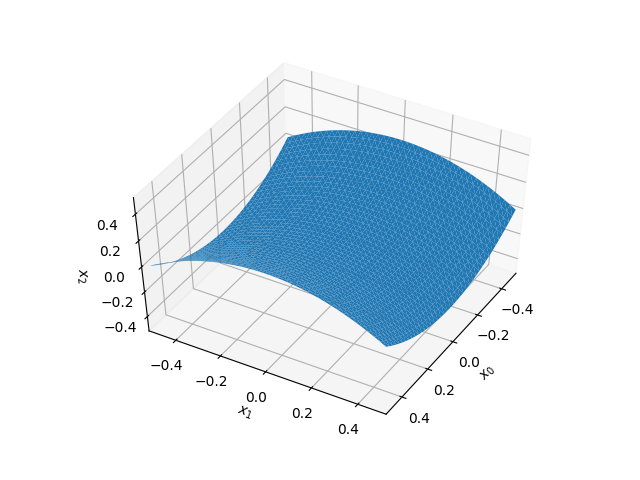
The midplane of the initial (stress-free) configuration \(\mathcal{S}_I\) of the shell is given in the form of an analytical expression
in terms of the curvilinear coordinates \(x\). Hence, we mesh the two-dimensional domain \(\mathcal{M}\equiv [-L/2,L/2]\times [-L/2,L/2]\).:
L = 1.0
P1, P2 = Point(-L/2, -L/2), Point(L/2, L/2)
ndiv = 40
mesh = RectangleMesh(P1, P2, ndiv, ndiv)
We provide the analytical expression of the initial shape as an
Expression that we represent on a suitable FunctionSpace (here
\(P_2\), but other are choices are possible):
initial_shape = Expression(('x[0]','x[1]','x[0]*x[0] - x[1]*x[1]'), degree = 4)
V_y = FunctionSpace(mesh, VectorElement("P", triangle, degree=2, dim=3))
yI = project(initial_shape, V_y)
We compute the covariant and contravariant component of the
metric tensor, aI, aI_contra; the covariant base vectors g0, g1;
the contravariant base vectors g0_c, g1_c.
aI = grad(yI).T*grad(yI)
aI_contra, jI = inv(aI), det(aI)
g0, g1 = yI.dx(0), yI.dx(1)
g0_c, g1_c = aI_contra[0,0]*g0 + aI_contra[0,1]*g1, aI_contra[1,0]*g0 + aI_contra[1,1]*g1
Given the midplane, we define the corresponding unit normal as below and project on a suitable function space (here \(P_1\) but other choices are possible):
def normal(y):
    n = cross(y.dx(0), y.dx(1))
    return n/sqrt(inner(n,n))

V_normal = FunctionSpace(mesh, VectorElement("P", triangle, degree = 1, dim = 3))
nI = project(normal(yI), V_normal)
We can visualize the shell shape and its normal with this utility function
def plot_shell(y,n=None):
    y_0, y_1, y_2 = y.split(deepcopy=True)
    fig = plt.figure()
    ax = fig.gca(projection='3d')
    ax.plot_trisurf(y_0.compute_vertex_values(),
                    y_1.compute_vertex_values(),
                    y_2.compute_vertex_values(),
                    triangles=y.function_space().mesh().cells(),
                    linewidth=1, antialiased=True, shade = False)
    if n:
        n_0, n_1, n_2 = n.split(deepcopy=True)
        ax.quiver(y_0.compute_vertex_values(),
              y_1.compute_vertex_values(),
              y_2.compute_vertex_values(),
              n_0.compute_vertex_values(),
              n_1.compute_vertex_values(),
              n_2.compute_vertex_values(),
              length = .2, color = "r")
    ax.view_init(elev=50, azim=30)
    ax.set_xlim(-0.5, 0.5)
    ax.set_ylim(-0.5, 0.5)
    ax.set_zlim(-0.5, 0.5)
    ax.set_xlabel(r"$x_0$")
    ax.set_ylabel(r"$x_1$")
    ax.set_zlabel(r"$x_2$")
    return ax

plot_shell(yI)
plt.savefig("output/initial_configuration.png")
In our 5-parameter Naghdi shell model the configuration of the shell is assigned by
- the 3-component vector field
u_representing the (small) displacement with respect to the initial configurationyI - the 2-component vector field
theta_representing the (small) rotation of fibers orthogonal to the middle surface.
Following [2, 3], we use a P2+bubble element for y_ and a P2
element for theta_, and collect them in the state vector
z_=[u_, theta_]. We further define Function, TestFunction, and
TrialFucntion and their different split views, which are useful for
expressing the variational formulation.
P2 = FiniteElement("P", triangle, degree = 2)
bubble = FiniteElement("B", triangle, degree = 3)

Z = FunctionSpace(mesh, MixedElement(3*[P2 + bubble ] + 2*[P2]))
z_ = Function(Z)
z, zt = TrialFunction(Z), TestFunction(Z)

u0_, u1_, u2_, th0_, th1_ = split(z_)
u0t, u1t, u2t, th0t, th1t = split(zt)
u0, u1, u2, th0, th1 = split(z)
We define the displacement vector and the rotation vector, with this latter tangent to the middle surface, \(\theta = \theta_\sigma \, g^\sigma\), \(\sigma = 0, 1\)
u_, u, ut = as_vector([u0_, u1_, u2_]), as_vector([u0, u1, u2]), as_vector([u0t, u1t, u2t])
theta_, theta, thetat = th0_*g0_c + th1_*g1_c, th0*g0_c + th1*g1_c, th0t*g0_c + th1t*g1_c
The extensional, e_naghdi, bending, k_naghdi, and shearing, g_naghdi, strains
in the linear Naghdi model are defined by
e_naghdi = lambda v: 0.5*(grad(yI).T*grad(v) + grad(v).T*grad(yI))
k_naghdi = lambda v, t: -0.5*(grad(yI).T*grad(t) + grad(t).T*grad(yI)) - 0.5*(grad(nI).T*grad(v) + grad(v).T*grad(nI))
g_naghdi = lambda v, t: grad(yI).T*t + grad(v).T*nI
Using curvilinear coordinates, the constitutive equations are written in terms
of the matrix A_hooke below, representing the contravariant components of
the constitutive tensor for isotropic elasticity in plane stress, see e.g.
[4]. We use the index notation offered by UFL to express operations
between tensors
i, j, k, l = Index(), Index(), Index(), Index()
A_hooke = as_tensor((((2.0*lb*mu)/(lb + 2.0*mu))*aI_contra[i,j]*aI_contra[k,l] + 1.0*mu*(aI_contra[i,k]*aI_contra[j,l] + aI_contra[i,l]*aI_contra[j,k])),[i,j,k,l])
The membrane stress and bending moment tensors, N and M, and shear
stress vector, T, are
N = as_tensor((A_hooke[i,j,k,l]*e_naghdi(u_)[k,l]),[i, j])
M = as_tensor(((1./12.0)*A_hooke[i,j,k,l]*k_naghdi(u_, theta_)[k,l]),[i, j])
T = as_tensor((mu*aI_contra[i,j]*g_naghdi(u_, theta_)[j]), [i])
Hence, the contributions to the elastic energy densities due to membrane,
psi_m, bending, psi_b, and shear, psi_s, are
psi_m = .5*inner(N, e_naghdi(u_))
psi_b = .5*inner(M, k_naghdi(u_, theta_))
psi_s = .5*inner(T, g_naghdi(u_, theta_))
Shear and membrane locking are treated using the PSRI proposed by Arnold and Brezzi, see [2, 3]. In this approach, shear and membrane energies are splitted as a sum of two weighted contributions, one of which is computed with a reduced integration. Thus, shear and membrane energies have the form
While [2, 3] suggest a 1-point reduced integration, we observed that this leads to spurious modes in the present case. We use then \(2\times 2\)-points Gauss integration for the portion \(\kappa - \alpha\) of the energy, whilst the rest is integrated with a \(4\times 4\) scheme. As suggested in [3], we adopt an optimized weighting factor \(\alpha = 1\)
dx_h = dx(metadata={'quadrature_degree': 2})
alpha = 1.0
kappa = 1.0/t**2
shear_energy = alpha*psi_s*sqrt(jI)*dx + (kappa - alpha)*psi_s*sqrt(jI)*dx_h
membrane_energy = alpha*psi_m*sqrt(jI)*dx + (kappa - alpha)*psi_m*sqrt(jI)*dx_h
bending_energy =  psi_b*sqrt(jI)*dx
Then, the elastic energy is
elastic_energy = (t**3)*(bending_energy + membrane_energy + shear_energy)
The shell is subjected to a constant vertical load. Thus, the external work is
body_force = 8.*t
f = Constant(body_force)
external_work = f*u2_*sqrt(jI)*dx
We now compute the total potential energy with its first and second derivatives
Pi_total = elastic_energy - external_work
residual = derivative(Pi_total, z_, zt)
hessian = derivative(residual, z_, z)
The boundary conditions prescribe a full clamping on the \(x_0 = -L/2\) boundary, while the other sides are left free
left_boundary = lambda x, on_boundary: abs(x[0] + L/2) <= DOLFIN_EPS and on_boundary
clamp = DirichletBC(Z, project(Expression(("0.0", "0.0", "0.0", "0.0", "0.0"), degree = 1), Z), left_boundary)
bcs = [clamp]
We now solve the linear system of equations
output_dir = "output/"
A, b = assemble_system(hessian, residual, bcs=bcs)
solver = PETScLUSolver("mumps")
solver.solve(A, z_.vector(), b)
u0_h, u1_h, u2_h, th0_h, th1_h = z_.split(deepcopy=True)
Finally, we can plot the final configuration of the shell
scale_factor = 1e4
plot_shell(project(scale_factor*u_ + yI, V_y))
plt.savefig("output/finalconfiguration.png")
References
[1] K. J. Bathe, A. Iosilevich, and D. Chapelle. An evaluation of the MITC shell elements. Computers & Structures. 2000;75(1):1-30.
[2] D. Arnold and F.Brezzi, Mathematics of Computation, 66(217): 1-14, 1997. https://www.ima.umn.edu/~arnold//papers/shellelt.pdf
[3] D. Arnold and F.Brezzi, The partial selective reduced integration method and applications to shell problems. Computers & Structures. 64.1-4 (1997): 879-880.
[4] P. G. Ciarlet. An introduction to differential geometry with applications to elasticity. Journal of Elasticity, 78-79(1-3):1–215, 2005.