Bifurcation of a composite laminate plate modeled with von-Kármán theory
This demo is implemented in the single Python file demo_von-karman-composite.py.
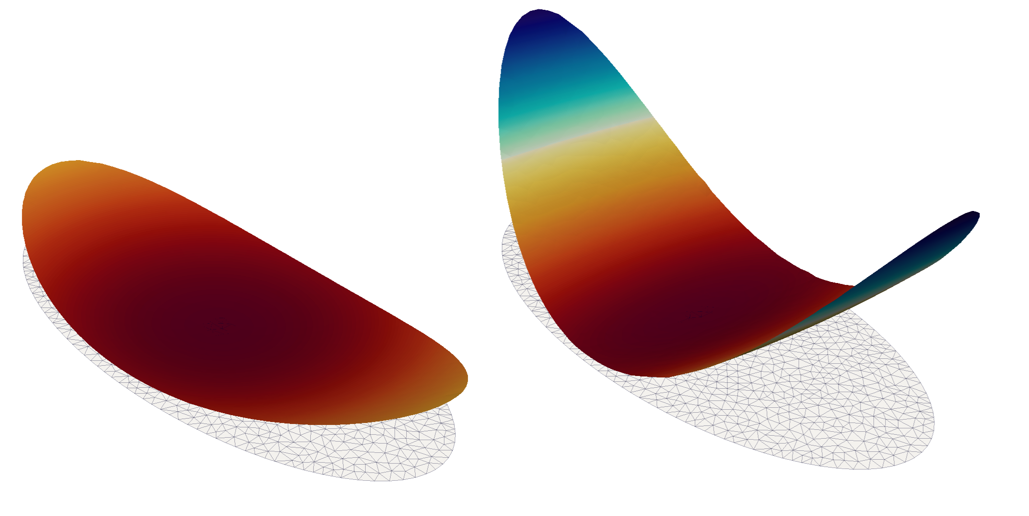
This demo program solves the von-Kármán equations for an elliptic composite plate with a lenticular cross section free on the boundary. The plate is heated, causing it to bifurcate. Bifurcation occurs with a striking shape transition: before the critical threshold the plate assumes a cup-shaped configurations (left); above it tends to a cylindrical shape (right).
An analytical solution can be computed using the procedure outlined in the paper [Maurini].
| [Maurini] | (1, 2) A. Fernandes, C. Maurini, S. Vidoli, “Multiparameter actuation for shape control of bistable composite plates.” International Journal of Solids and Structures. Vol. 47. Pages 1449-145., 2010. |
The standard von-Kármán theory gives rise to a fourth-order PDE which requires the transverse displacement field \(w\) to be sought in the space \(H^2(\Omega)\). We relax this requirement in the same manner as the Kirchoff-Love plate theory can be relaxed to the Reissner-Mindlin theory. Accordingly, we seek a transverse displacement field \(w\) in \(H^1(\Omega)\) and a rotation field \(\theta\) in \([H^2(\Omega)]^2\). To alleviate the resulting shear-locking issue we then apply the Durán-Liberman reduction operator.
To follow this demo you should know how to:
- Define a
MixedElementand aFunctionSpacefrom it. - Define the Durán-Liberman (MITC) reduction operator using UFL. This procedure eliminates the shear-locking problem.
- Write variational forms using the Unified Form Language.
- Use the fenics-shell function
laminate()to compute the stiffness matrices. - Automatically derive Jacobian and residuals using
derivative(). - Apply Dirichlet boundary conditions using
DirichletBCandapply(). - Assemble forms using
assemble(). - Solve linear systems using
LUSolver. - Output data to XDMF files with
XDMFFile.
This demo then illustrates how to:
- Define the Reissner-Mindlin-von-Kármán plate equations using UFL.
- Use the
ProjectedNonlinearSolverclass to drive the solution of a non-linear problem with projected variables.
We begin by setting up our Python environment with the required modules::
from dolfin import *
from ufl import RestrictedElement

from fenics_shells import *
import numpy as np

try:
   import matplotlib.pyplot as plt
except ImportError:
   raise ImportError("matplotlib is required to run this demo.")

try:
   import mshr
except ImportError:
   raise ImportError("mshr is required to run this demo.")
The mid-plane of the plate is an elliptic domain with semi-axes \(a = 1\)
and \(b = 0.5\). We generate a mesh of the domain using the package mshr:
a_rad = 1.0
b_rad = 0.5
n_div = 30

centre = Point(0.,0.)

geom = mshr.Ellipse(centre, a_rad, b_rad)
mesh = mshr.generate_mesh(geom, n_div)
The lenticular thinning of the plate can be modelled directly through the thickness parameter in the plate model:
h = interpolate(Expression('t0*(1.0 - (x[0]*x[0])/(a*a) - (x[1]*x[1])/(b*b))', t0=1E-2, a=a_rad, b=b_rad, degree=2), FunctionSpace(mesh, 'CG', 2))
We assume the plate is a composite laminate with 8-layer stacking sequence:
with elementary layer properties \(E_1 = 40.038, E_2=1, G_{12}=0.5, \nu_{12}=0.25, G_{23}=0.4\):
thetas = [np.pi/4., -np.pi/4., -np.pi/4., np.pi/4., -np.pi/4., np.pi/4., np.pi/4., -np.pi/4.]
E1 = 40.038
E2 = 1.0
G12 = 0.5
nu12 = 0.25
G23 = 0.4
We use our function laminates() to compute the stiffness matrices according to the Classical Laminate
Theory:
n_layers= len(thetas)
hs = h*np.ones(n_layers)/n_layers
A, B, D = laminates.ABD(E1, E2, G12, nu12, hs, thetas)
Fs = laminates.F(G12, G23, hs, thetas)
We then define our MixedElement which will discretise the in-plane
displacements \(v \in [\mathrm{CG}_1]^2\), rotations \(\theta \in
[\mathrm{CG}_2]^2\), out-of-plane displacements \(w \in \mathrm{CG}_1\).
Two further auxilliary fields are also considered, the reduced
shear strain \(\gamma_R\), and a Lagrange multiplier field \(p\) which
ties together the shear strain calculated from the primal variables
\(\gamma = \nabla w - \theta\) and the reduced shear strain
\(\gamma_R\). Both \(p\) and \(\gamma_R\) are discretised in
the space \(\mathrm{NED}_1\), the vector-valued Nédélec elements of the
first kind. The final element definition is then:
element = MixedElement([VectorElement("Lagrange", triangle, 1),
                        VectorElement("Lagrange", triangle, 2),
                        FiniteElement("Lagrange", triangle, 1),
                        FiniteElement("N1curl", triangle, 1),
                        RestrictedElement(FiniteElement("N1curl", triangle, 1), "edge")])
We then pass our element through to the ProjectedFunctionSpace
constructor. As we will see later in this example, we can project out both the
\(p\) and \(\gamma_R\) fields at assembly time. We specify this
by passing the argument num_projected_subspaces=2:
U = ProjectedFunctionSpace(mesh, element, num_projected_subspaces=2)
U_F = U.full_space
U_P = U.projected_space
Using only the full function space object U_F we setup our variational
problem by defining the Lagrangian of our problem. We begin by creating a
Function and splitting it into each individual component function:
u, u_t, u_ = TrialFunction(U_F), TestFunction(U_F), Function(U_F)
v_, theta_, w_, R_gamma_, p_ = split(u_)
The membrane strain tensor \(e\) for the von-Kármán plate takes into account the nonlinear contribution of the transverse displacement in the approximate form:
which can be expressed in UFL as:
e = sym(grad(v_)) + 0.5*outer(grad(w_), grad(w_))
The membrane energy density \(\psi_N\) is a quadratic function of the membrane strain
tensor \(e\). For convenience, we use our function strain_to_voigt() to express \(e\) in Voigt notation \(e_V = \{e_1, e_2, 2 e_{12}\}\):
ev = strain_to_voigt(e)
Ai = project(A, TensorFunctionSpace(mesh, 'CG', 1, shape=(3,3)))
psi_N = .5*dot(Ai*ev, ev)
The bending strain tensor \(k\) and shear strain vector \(\gamma\) are identical to the standard Reissner-Mindlin model. The shear energy density \(\psi_T\) is a quadratic function of the reduced shear vector:
Fi = project(Fs, TensorFunctionSpace(mesh, 'CG', 1, shape=(2,2)))
psi_T = .5*dot(Fi*R_gamma_, R_gamma_)
The bending energy density \(\psi_M\) is a quadratic function of the bending strain tensor. Here, the temperature profile on the plate is not modelled directly. Instead, it gives rise to an inelastic (initial) bending strain tensor \(k_T\) which can be incoporated directly in the Lagrangian:
k_T = as_tensor(Expression((("1.0*c","0.0*c"),("0.0*c","1.0*c")), c=1.0, degree=0))
k = sym(grad(theta_)) - k_T
kv = strain_to_voigt(k)
Di = project(D, TensorFunctionSpace(mesh, 'CG', 1, shape=(3,3)))
psi_M = .5*dot(Di*kv, kv)
Note
The standard von-Kármán model can be recovered by substituting in the Kirchoff constraint \(\theta = \nabla w\).
Finally, we define the membrane-bending coupling energy density \(\psi_{NM}\), even if it vanishes in this case:
Bi = project(B, TensorFunctionSpace(mesh, 'CG', 1, shape=(3,3)))
psi_MN = dot(Bi*kv, ev)
This problem is a pure Neumann problem. This leads to a nullspace in the solution. To remove this nullspace, we fix the displacements in the central point of the plate:
h_max = mesh.hmax()
def center(x,on_boundary):
    return x[0]**2 + x[1]**2 < (0.5*h_max)**2

bc_v = DirichletBC(U.sub(0), Constant((0.0,0.0)), center, method="pointwise")
bc_R = DirichletBC(U.sub(1), Constant((0.0,0.0)), center, method="pointwise")
bc_w = DirichletBC(U.sub(2), Constant(0.0), center, method="pointwise")
bcs = [bc_v, bc_R, bc_w]
Finally, we define the Durán-Liberman reduction operator by tying the shear strain calculated with the displacement variables \(\gamma = \nabla w - \theta\) to the conforming reduced shear strain \(\gamma_R\) using the Lagrange multiplier field \(p\):
gamma = grad(w_) - theta_
L_R = inner_e(gamma - R_gamma_, p_)
We can now define our Lagrangian for the complete system:
L = (psi_M + psi_T + psi_N + psi_MN)*dx + L_R
F = derivative(L, u_, u_t)
J = derivative(F, u_, u)
The solution of a non-linear problem with the ProjectedFunctionSpace
functionality is a little bit more involved than the linear case. We provide a
special class ProjectedNonlinearProblem which conforms to the
DOLFIN NonlinearProblem interface that hides much of the
complexity.
Note
Inside ProjectedNonlinearProblem, the Jacobian and residual
equations on the projected space are assembled using the special assembler
in FEniCS Shells. The Newton update is calculated on the space U_P.
Then, it is necessary to update the variables in the full space U_F
before performing the next Newton iteration.
In practice, the interface is nearly identical to a standard implementation of
NonlinearProblem, except the requirement to pass a
Function on both the full u_ and projected spaces u_p_:
u_p_ = Function(U_P)
problem = ProjectedNonlinearProblem(U_P, F, u_, u_p_, bcs=bcs, J=J)
solver = NewtonSolver()
solver.parameters['absolute_tolerance'] = 1E-12
We apply the inelastic curvature with 20 continuation steps. The critical
loading c_cr as well as the solution in terms of curvatures is taken from the analytical solution. Here, \(R_0\) is the scaling radius of curvature and \(\beta = A_{2222}/A_{1111}=D_{2222}/D_{1111}\) as in [Maurini]:
from fenics_shells.analytical.vonkarman_heated import analytical_solution
c_cr, beta, R0, h_before, h_after, ls_Kbefore, ls_K1after, ls_K2after = analytical_solution(Ai, Di, a_rad, b_rad)
cs = np.linspace(0.0, 1.5*c_cr, 20)
We solve as usual:
domain_area = np.pi*a_rad*b_rad
kx = []
ky = []
kxy = []
ls_load = []

for i, c in enumerate(cs):
    k_T.c = c
    solver.solve(problem, u_p_.vector())
    v_h, theta_h, w_h, R_theta_h, p_h = u_.split()
Then, we assemble the bending strain tensor:
k_h = sym(grad(theta_h))
K_h = project(k_h, TensorFunctionSpace(mesh, 'DG', 0))
we calculate the average bending strain:
Kxx = assemble(K_h[0,0]*dx)/domain_area
Kyy = assemble(K_h[1,1]*dx)/domain_area
Kxy = assemble(K_h[0,1]*dx)/domain_area

ls_load.append(c*R0)
kx.append(Kxx*R0/np.sqrt(beta))
ky.append(Kyy*R0)
kxy.append(Kxy*R0/(beta**(1.0/4.0)))
and output the results at each continuation step:
save_dir = "output/"
fields = {"theta": theta_h, "v": v_h, "w": w_h, "R_theta": R_theta_h}
for name, field in fields.items():
    field.rename(name, name)
    field_file = XDMFFile("{}/{}_{}.xdmf".format(save_dir, name, str(i).zfill(3)))
    field_file.write(field)
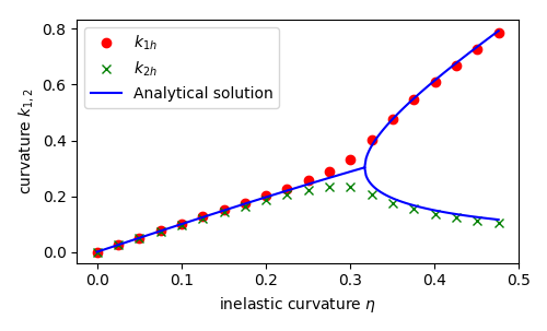
Finally, we compare numerical and analytical solutions:
fig = plt.figure(figsize=(5.0, 5.0/1.648))
plt.plot(ls_load, kx, "o", color='r', label=r"$k_{1h}$")
plt.plot(ls_load, ky, "x", color='green', label=r"$k_{2h}$")
plt.plot(h_before, ls_Kbefore, "-", color='b', label="Analytical solution")
plt.plot(h_after, ls_K1after, "-", color='b')
plt.plot(h_after, ls_K2after, "-", color = 'b')
plt.xlabel(r"inelastic curvature $\eta$")
plt.ylabel(r"curvature $k_{1,2}$")
plt.legend()
plt.tight_layout()
plt.savefig("curvature_bifurcation.png")
Unit testing
import pytest
@pytest.mark.skip
def test_close():
    pass